

With rapid growth in usage of mobile applications worldwide, we have to deal with rapidly increasing data as well. For the ad tech companies, identifying unique users with particular interest provided by the advertiser in the demand side is a cumbersome process as we need to query on tera bytes of data available worldwide. In this situation, there are several use cases to consider like:
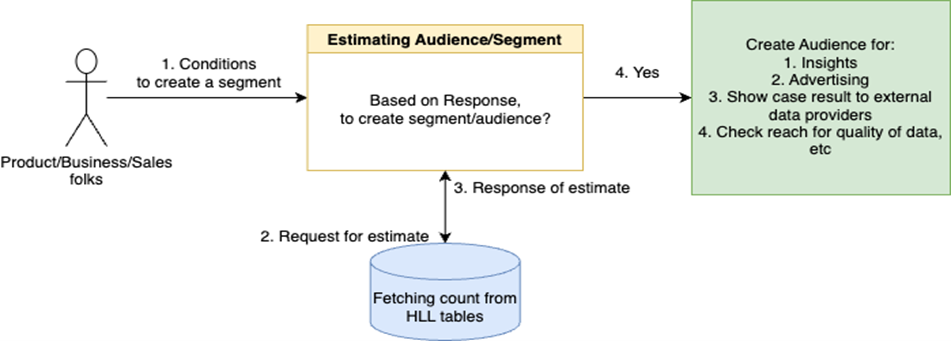
Campaign managers can create segments/audience with better reach.
Sales managers can showcase our supply data quality to clients.
Brand managers can run marketing campaigns with better understanding of their users.


For all the above cases, a quick count on terabytes of data is required to deliver and check on segment quality or sizing. If calculating the total count of such people takes time, then it may lose the confidence of the advertiser to even broadcast their ad, or the advertiser can get their request filled on other ad tech companies and run campaigns on mobile applications, or the sales manager could lose bids or contracts between the advertiser and ad campaigns. To build an algorithm/solution where we can quickly estimate on terabytes of data as per the conditions provided from the advertiser in few seconds only with minimal resources to avoid hardware cost as well.
An audience or segment is a list of users that satisfy some conditions, for example, female users aged 18-34 or male users who visited McDonalds/KFC, USA in last the 2 weeks. These segments participate in auctions and add more revenue if the advertiser requests to start the campaign.


Whenever these requests arrive, we need to calculate all such users provided with the conditions. These requests are easy to process, but they get queried on terabytes of data which requires good hardware resource that can filter out conditions on full-scaled data and then provide us with the sum of unique users.
Let’s compare HLL with the original data with respect to data size, query time, and result.
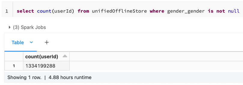
Machine used: 64 GB, 16 cores – 1 node.
Query time: 7 hours, Data format: ORC, Size of data: ~ 3 TB
Query time: 0.66 seconds, Data format: Delta, Size of data: ~ 90 MB
It’s clearly visible that if we get such small requests on big data then it get too difficult to query on data. To get faster results we need to scale up our resources significantly that would incur huge costs.
With such requests we need to ensure that:
The hardware resources are always up and running.
There is enough scaling so that parallel request can be achieved.
The data is always available.
There is no memory failure.
Even after ensuring all of the above there is still no guarantee that an advertiser will select the segment for their campaign as there could be reasons like:
There is not enough scale of users.
An advertiser finds another DSP with their request fulfilled.
In any case hardware cost will be incurred to fetch the segment. Being a very specific segment, there will be little or no requirement from other advertisers as they may not even belong to that segment.
In these situations, we need to build a solution where we could query data in seconds with minimal hardware that would eventually:
Save hardware costs.
Figure out scale of a segment quickly.
Avoid scenarios where advertisers need to wait for long.
HLL stands for HyperLogLog, which is an algorithm to solve for count-distinct problem. It approximates the number of unique elements in your data and can convert dimension to measure. It comes with the ability to merge (union) together two different sets. The algorithm assigns Sketch which gives us probabilistic data structure that converts data to binary value based on the hash value provided to it which in turn processes and helps in searching large amount of data very fast. Since it uses hash values it loses some accuracy to each unique element in the set. We can easily merge the Sketch with other dimension properties resulting in lesser rows altogether.
Suppose that we have millions of user ids and their gender corresponding to each of them. Here the user id will get converted to a Sketch (which is nothing but a hash value that the HLL algorithm generates), which will further be aggregated and result in just two rows for each gender and corresponding to them there will be a merged Sketch. The change from a million to just two rows have reduced the data exponentially, and the query time will now be in milliseconds. All you need now is cardinality of each gender.
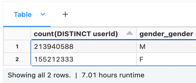
The following is the original table:
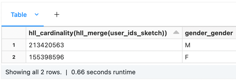
The following is the HLL table:
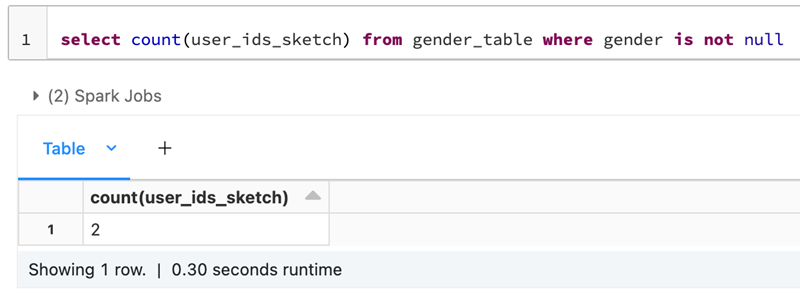
It’s clearly visible that all the 1.3 billion gender rows are merged into two in the HLL table, where one row depicts male while the other female.
In our use case we need:
A quick approximate count for a segment requested by an advertiser.
Insights on a segment/audience, brand, POI, residence etc., (for example, user insights like gender split, age split, location insights out of a segment quickly, or insights on people visiting a specific brand).
Merging and intersecting between segments (or say sets).
As all above use cases requires count-distinct problem to solve in an efficient and faster way, hence HLL seems to be a promising solution.
HLL algorithm comes along with cardinality and merging (union) between sets, and in our use case we require intersection operation as well. Other Sketches are also available like the Theta Sketch that we used earlier to have both intersection and union, but its size grows in an increment of 8 bytes while HLL grow in 4 bytes. Though Theta Sketch solved most of our problems, but more optimizations were still needed, and using HLL was our first optimization. HLL Sketches can be 2-16 times smaller for the same accuracy compared to Theta Sketches, and the intersection operation can be simply solved by the famous Principle of Inclusion and Exclusion property.
n (A n B) = n(A) + n(B) – n (A u B)
In above formula, we know that on the right-hand side of the formula, the cardinality of A and B as element and union of them is already provided by HLL. We received the cardinality of elements and performed elementary arithmetic operation on them.
As we can merge (union) n number of statements in HLL, there was a requirement to intersect multiple statements. In our use case sales/business folks might intersect between multiple statements to find users of common interest.
Similarly, a generalized formula is designed in the HLL algorithm where we can get intersection result for n number of sets. In the HLL algorithm, as we get cardinality and merge operation and using these two operations in the right-hand side of formula in 1, intersection cardinality can be achieved and with this we have solved problem like n (a1 n a2 n a3 n a4 n…), where ai is the number of sets.
The library to implement HLL have HLL functions which requires Spark as session and hence they will only be available when our Databricks cluster is up and running to get the park session available to the library, and since the Spark session is not available via JDBC connection, the functions were just only being able to call via Databricks APIs.
We solved this problem by implementing Spark Extensions which facilitates us to add functions to Spark without calling or merging the functions with Spark. This extension helps us with calling the HLL functions via JDBC connection.
The second problem with HLL is the extension of above problem only where if a user queries with multiple intersection and union operation in one statement.
(A n B) u C
For a use case like the above, there can be any combination between sets a user can query.
We solved this by converting Disjunctive Normal Form (DNF) to Conjunctive Normal Form (CNF). Here, a generalized logic has been implemented to convert the DNF to a form where the sets operations will be done by intersection.
(A n B) u C = (A u C) n (A u C) → (A1 n B1)
Now every valid form can be converted to a form where resultant sets will be intersection among them.
Our offline store for the supply-side platform (SSP) stores user activities and their attributes for 13 months. For estimation (and segmentation later), we are interested only in the last 3 months of data. It's a user pivoted store, and the data contains several feature groups, representing different families of information like demographics, location timeline, app usage timeline etc.
The schema consists of following feature groups:
Age
Gender
Carrier information
Handset information
App information
OS information
Point of interest information
Polygon information
Region information
Apps install/uninstall behavior information
The above feature groups combined act as a single table and all these groups have 2-8 sub columns to it, which in total results in around 40 columns along with user id (which in our case will act as HLL sketch).
The above schema is partitioned by two layers.
Time Variant Data: Where user feature groups keep changing such as POI, App, Polygon & Region, and Install & Uninstall behavior of apps.
Non Time Variant Data: This concerns all the static data.
These feature groups are mapped to the individual users.
The table was flattened in structure so that these feature groups are no longer there, and the table was populated keeping one feature group as fixed and rest other as null with the user id. Keeping additive property instead of multiplicative property, for example, if we have gender set cardinality to be 2 and POI cardinality to be 500 ids then the resulting table would have 500x2 rows while performing aggregation, but as HLL the problem can be solved by treating gender and POI as set and performing intersection between them to get the same result. We populated the data as 500 sketch ids of POI + 2 sketch ids of gender with merged user id sketch.
1 month of flat SSP data of 1.5 TB size was reduced to around 30 GB of data.
Query time was reduced from 30-120 mins query to 2-5 minutes (max) with 4 nodes of 12 core of each machine.
There was further scope of optimizing the above scenario by treating each feature group as individual table instead of having them in one table. In the optimization 1 scenario, the query in above table among different feature groups requires intersection operation. This intersection operation can work among different tables as well as user-id corresponds to each feature group.
30 GB of 1-month HLL table was now reduced to 12 GB of data (summation of each and individual group).
Query time was reduced from 2-5 minutes to 20-80 seconds (max) with 1 node of 8 core machine.
The above two optimization was acceptable in our case, but there was another scope of optimization in the resulted HLL table. The above resultant table can be further improved by sorting the data. Each feature group has ids corresponds to it, if the data gets sorted then data fetching from the table can be easy. Z-ordering is one of the features that we get in Databricks. Z-ordering sorts of the data in the order that we provide while optimizing the data. It maintains a file stats, so that there is no requirement to traverse the table files and it can directly point to the designated location.
Z-ordering colocates the related information together in same set of files. Here we provide the order of columns based on which the data will be sorted and stored.
The delta table has file level stats about each column. After having the column in order and sorted, whenever a query arrives with the stats, the files which are not required are skipped and the query just surfs the useful file as per our query.
Z-ordering creates new set of sorted and compacted files which are easier to loop up instead of having more set of unsorted files.
Query time was reduced from 20-80 seconds to 2-60 seconds (max) with 1 node of 8 core machine.
| 1 Month of User Data | Data Size | Machine Used | Query Time |
|---|---|---|---|
| Original Data | 1.5 TB | 64GB, 16 core – 4 nodes | 50-120 minutes |
| Optimization 1 – Generation of HLL table | 30 GB | 64GB, 16 core – 4 nodes | 2-5 minutes |
| Optimization 2 – Division of HLL table | 12 GB | 32GB, 8 core – 1 node | 20-120 seconds |
| Optimization 3 – Z-ordering on the table | 12 GB | 32GB, 8 core – 1 node | 2-60 seconds |


Sign up with your email address to receive news and updates from InMobi Technology


