
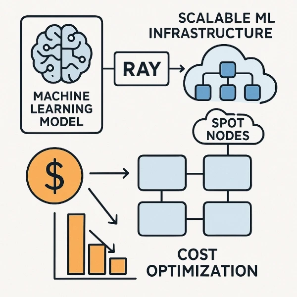
When it comes to machine learning (ML) training, cost and performance often go head-to-head. You want to train large models quickly, but you don’t want to break the bank. That’s where running Ray jobs on Spot Instances can shine—Spot Nodes are (usually) way cheaper, sometimes up to a 90% discount, compared to regular on-demand VMs. The tradeoff? Spot eviction during training leads to recomputations and can end up in a perpetual cycle of re-computation.
The primary challenge is balancing the cost savings while ensuring your training job isn’t stalled by too many spot evictions.
Ray is built around a cluster architecture consisting of a head node (which orchestrates task scheduling and cluster state) and worker nodes (which execute the distributed tasks). In the context of ML training, Ray provides abstractions such as Ray Train that handle data parallelism by distributing tasks (batches of data) across multiple worker nodes. One of its core synchronization methods, particularly in many training loops, is all-reduce, where gradients from each worker need to be combined and redistributed so that every node has the latest model parameters before proceeding to the next batch or epoch.
1. Worker Availability:
Because of Ray’s all-reduce mechanism, every active worker node is required for synchronization at the end of each training step. If a Spot node is evicted (terminated by the cloud provider on short notice), training stalls until Ray can either replace that node or reschedule the workload. This can lead to significant idle time while the cluster is waiting to return to a fully operational state.
2. Increased Overhead:
When a Spot node disappears, Ray needs to spin up a new worker on an available node. This process includes scheduling overhead, data reloading, and possibly re-initializing model weights from a checkpoint. Each interruption adds extra steps to the training loop, causing delays and sometimes repeated computation.
3. Potential Deadlocks:
If Spot evictions happen frequently, there could be extended periods when Ray can’t gather all workers simultaneously for the allreduce step. In worst-case scenarios, the job remains stuck, repeatedly attempting to restore lost workers, leading to deadlock-like conditions where progress is stalled indefinitely.
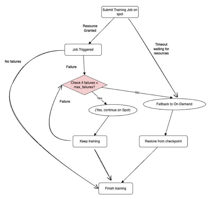
Given the unpredictability of Spot Instance availability, relying solely on them can lead to deadlocks in distributed training scenarios. Implementing a fallback mechanism ensures that if Spot Instances become unavailable or are interrupted too frequently, the workload can transition to more stable, albeit more expensive, regular instances, thereby maintaining the continuity of the training process. Ray’s fallback strategy makes sure that if Spot Instance failures occur too often, your training doesn’t stay stuck forever. We define a max_failures value in the scaling configuration, which tracks how many worker pods can fail, due to evictions or any other reason, before halting the Spot-based run. Once this threshold is reached, the training job stops and automatically restarts on on-demand nodes using the latest checkpoint, so you don’t lose progress. The value of max_failures can be set to -1 if you want to stay on Spot Instances indefinitely, no matter how many evictions occur.
Checkpointing is a fundamental building block of any fault-tolerant ML training pipeline, especially when using unreliable infrastructure like Spot instances. It ensures that progress is not lost when failures occur. In distributed training, a single worker node failure (e.g., due to Spot eviction) can cause the job to crash. Without checkpointing, you’d need to start from scratch, wasting compute time and cost. Checkpointing allows the job to resume from the last saved state, preserving training progress even across interruptions and resource switches.
When max_failures is hit and the job transitions from Spot to On-Demand, Ray restores the job from the latest checkpoint, continuing seamlessly. This avoids repeating epochs or recomputing gradients, ensuring both efficiency and consistency in results.
In TensorFlow, checkpointing is typically handled using the tf.train.Checkpoint API. This integrates smoothly with Ray, which can track and persist these checkpoints if you report them using train.report() inside your training loop.
1. Save frequently, ideally after every N batches or epochs.
2. Store in shared/durable storage (e.g., S3, Blob, NFS) to survive node failures.
3. Ensure consistency: save all training-related state—model, optimizer, learning rate scheduler, etc.
In distributed machine learning (ML) training, especially when utilizing spot instances, ensuring fault tolerance is crucial due to the potential for unexpected interruptions. While frameworks like Ray and TensorFlow offer foundational tools to address these challenges, integrating their functionalities requires a customized approach to create an effective fallback mechanism.
When to fallback
1. Eviction/max_failures: We can fallback to On-demand nodes in case we have seen enough failures/evictions on spot nodes.
2. Timeout due to unavailability: If the nodes are not present at all to start the job or cannot procure nodes after eviction, a timeout should be configured to avoid an infinite wait.
Understanding the Components:
1. Ray’s max_failures Parameter:
Ray provides the max_failures setting within its FailureConfig, allowing users to define the number of permissible recovery attempts for a training run. Upon reaching this threshold, Ray will halt the job.
2. Checkpointing with TensorFlow:
TensorFlow facilitates the saving of a model’s state through its checkpointing capabilities. Training can resume from the last saved state after an interruption by periodically capturing the model's parameters.
3. Ray’s Restore Functionality:
Ray’s Tuner.restore method enables the resumption of a previously failed run from its last checkpoint. This function is essential for continuing training without starting over.
By combining Ray’s failure handling and restoration features with TensorFlow’s checkpointing, a robust fallback mechanism can be developed:
Checkpoint Utilization: Implement TensorFlow’s checkpointing to save the model’s state at regular intervals, ensuring that training progress is preserved.
Job Restoration with Modified Configuration: Upon job termination due to reaching the failure threshold, use Ray’s Tuner.restore function to restart the job from the last checkpoint. Modify the job’s configuration to switch from spot instances to on-demand instances, thereby enhancing stability.
This integrated approach allows for the seamless transition between different instance types, ensuring that training processes are resilient to spot instance interruptions and can continue with minimal disruption.
Setting a higher max_failures value allows the training job to tolerate more interruptions, which is beneficial when utilizing spot instances prone to preemption. However, each interruption necessitates a recovery process, including restarting tasks and reloading data, which extends the overall runtime. While this approach maximizes the use of cost-effective spot instances, it may lead to longer training durations due to the cumulative effect of handling multiple failures.
Assumptions:
To establish a consistent baseline for analysis, we consider the following assumptions:
| Symbol | Meaning |
| T | Total job time (in hours) if fully run on On-Demand nodes |
| α | Fraction of the job that runs on Spot nodes before fallback |
| M | max_failures: Number of Spot interruptions tolerated before fallback |
| Δt | Overhead (in hours) added per Spot failure (restart, reschedule, etc.) |
| Cₒ | On-Demand cost per hour |
| Cₛ | Spot cost per hour = 0.1 × Cₒ (i.e., 90% discount) |
| S | Final cost savings percentage |
We decompose the total runtime into:
Here are the equations with the requested formatting changes:
TS = α * T
TO = (1 - α) * T + M * Δt
Ttotal = T + M * Δt
This shows how higher max_failures allow more progress on Spot but increase the total time due to accumulated restart overhead.
The total cost of the training job when using Spot and fallback is:
Cfallback = TS * CS + TO * CO
The baseline cost if the entire job ran on On-Demand:
Cold = T*CO
Assuming CS = (0.1) * CO, we derive the cost savings as:
Cnew = α * (0.1*CO) * Ttotal + (1 - α) * (CO) * Ttotal
Cnew = (T + M * Δt) * CO * (1 - 0.9*α)
This clean expression cost as a function of three critical design variables:
Cnew = Ttotal * CO * (1 - 0.9*α)
Cold = T * CO
Hence, cost saving will happen if below equation satisfies
Ttotal * (1 - 0.9*α) < T
Runtime flexibility
| Job on Spot (%) | Runtime Flexibility (without cost increase) | Insight |
| 30% | Up to 36% longer runtime | Cost-efficient even with moderate Spot usage |
| 40% | Up to 56% longer runtime | High tolerance to delay, solid savings window |
| 50% | Up to 81% longer runtime | Break-even shifts significantly in your favor |
| 60% | Up to 217% longer runtime | Massive buffer—ideal for cost-optimized training jobs |
Let’s assume:
Cnew = Ttotal * CO * (1 - 0.9*α)
Cnew = 2.76CO
Savings = 5CO - 2.76CO = 2.24CO = 44.8% savings
So, even with 5 interruptions adding ~1 hour of overhead(20%), you still save around 45% of the cost compared to running the entire job on On-Demand instances.
Below are a few things to keep in mind while using the approach
| Parameter | Increase Effect |
| α ↑ | More Spot usage → higher savings |
| M ↑ | More tolerated failures → more savings, but higher runtime overhead |
| Δ t ↑ | Cost of failure grows → savings drop |
| T ↑ | Larger jobs tolerate failure better (savings drop less) |
This formula can be used as a design tool:
The above technique is not limited to spot to on-demand fallback, but can also extend to a general fallback scenario. You can have a list of machine types you want to use in any order, ensuring a sequential fallback happens based on thresholds, timeout, and other criteria. Selection of these machines can be multiple spot, on-demand, cross-region, etc., to ensure the reliability of the job.
With controlled thresholds (max_failures) and strategic checkpointing, fallback allows aggressive use of Spot resources without jeopardizing job completion.
Optimal settings depend on Spot market stability, model training duration, and checkpoint frequency. Fine-tuning this parameter ensures maximum savings without sacrificing reliability.
with minimal added runtime overhead, provided Spot interruptions are managed effectively.
In closing, the fallback mechanism we’ve discussed is more than a workaround—it’s a scalable pattern for building resilient, cost-optimized ML pipelines in cloud-native environments.
If you’re training large models regularly, this design could mean the difference between sustainable experimentation and budget overruns.
Handling Failures and Node Preemption — Ray 2.44.1
ray.tune.Tuner.restore — Ray 2.44.1


Sign up with your email address to receive news and updates from InMobi Technology